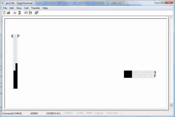
Figure 1: Image of the GUI for the default 2-dimensional application; the system is executing a "down" maneuver in the "Y" dimension,
while holding steady in the "X" dimension.
Introduction
The article at hand describes a set of techniques for the construction of networks of one or more Microchip Technology "PIC"
8-bit microcontrollers, in which each processor exercises cybernetic control over a single dimension (or degree
of freedom) using a PID (Proportional - Integral - Differential) control algorithm.
A complex control application, such as a robot, consists of several such PID control loops. These can run in parallel with each other, as is seen in the demonstration circuit
built for this article. In this circuit, an "X" dimension and a "Y" dimension are controlled, using similar means, but independently of each other.
It is also possible to connect control loops in series. On many boats and aircraft, for example, the task of controlling vehicle heading can be modeled by a PID loop commanding
rudder position. The heading control PID loop's output is a rudder position (e.g., in degrees), selected in an effort to achieve a user-designated heading setpoint. The positioning
of the vessel's rudder, though, often requires cybernetic control in its own right; the physical hardware may expose the ability to move the rudder to the right, or to the left,
for example, along with giving the ability to sense rudder position, without exposing any way to directly command a specific rudder position. It is in such situations that the concept
of connecting control loops in series becomes relevant.
A real cybernetic control application can thus rely on many control loops, and to be able to subdivide a complex control system in a one-processor-per-loop manner offers considerable
appeal. A one-loop-per-CPU design like the one presented in this article provides an easy answer to many design questions
that would otherwise accompany a concurrent multiprocessor system like the one described in this article. It is not easy to take a real problem and subdivide it definitively among
a handful of CPUs. Any architecture that offers this prospect deserves, the author hopes, a second glance.
The article at hand demonstrates that this simple, dimension-per-CPU approach to parallelism can indeed be made to work very well. A full hardware implementation is described,
and it is one that exercises obvious control over movement toward a setpoint in two dimensions, and does so in a way that is robust with respect to changes in the physical system.
Its scalability has been tested to 32 user-visible degrees of freedom, and basically unlimited internal PID loops. A man-machine interface based on an ANSI terminal GUI and an analog
joystick is provided.
The parallelism system employed here (one processor per control loop) is admirably simple; but one risk in anything so simple as the parallelism scheme just described is that
it will become overly simplistic. It is demonstrated below that, in many obvious ways, at least, this is not the case here.
A simplistic design can betray itself in several ways. Most obviously, it is possible that such a design will simply not function well, but the demonstration device built
in the article holds position well, and adapts admirably to environmental change. When powered on, for example, the demo application motor quickly and accurately moves its main
sliding assembly to the default position, and subsequent position moves commanded by the joystick are obeyed in similar fashion. This works well on some disparate hardware,
even before tuning constants (which are floating-point values) are adjusted. The associated man-machine interface is simple but intuitive and graphical, and is reliably rendered
at a high - and deterministic - frame rate of 6 frames-per-second.
From a specification standpoint, the analog inputs and outputs associated with the control system have a 10-bit resolution, the serial I/O performed by the processors occurs
at the RS-232 spec maximum of 115,200 baud, all PID calculations are done using floating-point numbers, and the system can be cheaply and quickly tuned in the field using
floating-point constants.
Beyond superficial performance, and beyond nominal specifications, though, an overly simplistic design can carry with it economic problems. Most design processes can simply buy
adequate performance using hardware overkill, but this is not the approach taken here. To say that doing all of the things described above using one PIC processor per control loop
seems like a very efficient result is a subjective assessment. This assessment, though, is one that more objective measures support. There is simply not much wasted space in this
design. A single PIC 16F690 cannot be expected to control more than one motor of the bi-directional sort used here, for example, because it cannot be configured to output two different
analog signals at once. For one such device to handle everything related to a single PID loop therefore does represent full employment of the device, from a standpoint of analog output count.
Furthermore, the 4 kiloword program memory of each PIC is over 90% filled by the code presented; several floating point operators are implemented in 8-bit machine language in support of the controller itself, and the largely 16-bit algorithms required are implemented in 8-bit PIC assembly language. This is an assembly language that lacks hardware multiply and divide instructions.
The existence of such an application using 8-bit PICs is, the author hopes, impressive; the prospect of being able to multiplex said application in scalable fashion is,
it is further hoped, even more impressive. It is also hoped that the economic implications of doing so using microcontrollers that retail at well under $2.00 per unit (along with some
cheaper discrete components) are especially impressive.
Finally, readers can rest assured that the design offered here rests on solid theoretical foundations already laid by the same author. As discussed in the next section,
the scalable architecture offered here derives from two key components: the very well-tested SFP real number type,
and the "Scrapnet" synchronous network. Each of these components receives an extensive and rigorous treatment
in its own article. Here, suffice it to say that both of these free components1 exemplifies the deterministic nature
of PIC code - even PIC code exhibiting substantial parallelism, and that this is a design direction which is expanded in this latest submission.
Background
To develop an application like this one from the integrated circuits up requires a great deal of underlying low-level work. The floating-point data type used here, "SFP",
and the operator functions required, are documented in this predecessor article. The multiprocessor serial networking scheme
employed, "Scrapnet", was similarly presented in another previous submission. The circuit presented here is a direct expansion of the circuit
shown in that article.
"Scrapnet" itself was an expansion of yet another article, where the real basics of wiring a PIC to a terminal are presented. In the interest
of brevity, the most basic of setup questions are better-addressed in these articles than they are here.
Using the Code
The GUI provided is shown in the first picture presented above. It is based around two bar graphs per dimension: one with the label "S" (for "Setpoint"),
which shows where the user commands the demo assembly to position itself, and another bar graph with the label "P" ("Position"), which shows the current actual position.
The joystick is used to make changes to the setpoint. If the joystick is held toward the right, for example, the horizontal "S" bar graph will move to the right in response,
and "P" will follow (if everything is working) as the motor control system causes the system position to move toward the setpoint.
The GUI code provided is designed for broad applicability. In the full two-PIC demonstration, the left CPU (if one views the circuit board with the processors' "pin 0"
at the front) renders a GUI based on vertical bar graphs, while the other CPU renders one that uses horizontal bar graphs. These are based on the 0 to 1023 range output by the 10-bit DAC,
with provisions for scaling the range of the bar graph to match the real range of position values attainable. Of course, in many practical applications this simple, general approach will
not be adequate. The 0 to 1023 range might need to be scaled to match user expectations. A 0-360 degree range would most likely be appropriate for a heading controller, for instance, perhaps
in conjunction with a circular, compass-like presentation. A simple rudder positioning system might have a GUI very similar to the one provided here, although even in this case some
concept of a center point would need to be introduced.
The "Scrapnet" protocol assigns a station number to each participating processor, based on the order (in the timer 1 period) in which the processors transmit.
In the demo application, the left processor is station 0 and the right processor is station 1. In general, each CPU in a complex control application implemented using the architecture
described here will run a PID loop, but only the CPUs that render a portion of the application GUI will have a "Scrapnet" station number. For example, in a serial control
loop application, the GUI might show graphics related to vessel heading, but not show graphics directly show rudder position. As detailed in the introduction, though, the rudder
positioning task would likely have a dedicated CPU - and control loop of its own - in such an application.
A reader interested in actually constructing the demonstration circuit should begin by following the (very detailed) instructions in this article
to get a basic PIC-to-terminal serial link working. This article also goes over issues of notation, especially as they relate to schematic diagrams and more details "rat's
nest" diagrams.
Subsequently, a reader engaged in the construction of the demo circuit described in this article must construct the demonstration board described
in the "Scrapnet" article. This article describes how to set up a grouping of PICs sharing a common clock and a common serial bus,
and gives a "rat's nest" diagram for a two-PIC demonstration board, along with source files for the necessary firmware for each processor. The photoresistor specified
in the "Scrapnet" demo should be omitted; in the control application described in this latest article, a second joystick axis is connected in its place.
The "rat's nest" format used in the "Scrapnet" article, and continued here, models a widely-available breadboard configuration (Radio Shack Part No. 276-002).
Other necessary supplies include jumper wires; Radio Shack part no. 276-173 is a suitable jumper wire kit. A 12 megahertz oscillator, an analog joystick, a PIC programmer, and some
diodes, resistors, and (for the full demo) capacitors are also necessary. These are all fairly commonplace items, but specific suggestions for their acquisition are given
in the "Scrapnet" article, where applicable, or later in this article.
The Radio Shack jumper wire kit closely matches the suggested breadboards. The kit contains wires of assorted length which can simply be pushed into the breadboard's holes
to make a connection. Connections of two sorts can be made. For a neat layout, the jumper wires can be laid flat against the breadboard. In dense areas of the circuit, these
connections are oriented mostly at right angles to its rows of holes. If this is done, and the wires are not crossed over each other, the resultant connections can be translated
into signal paths on a single-layer PCB (printed circuit board). Occasionally, though it will prove helpful
to make some long or problematic connection using a true jumper wire, i.e. one that protrudes up in the air in messy fashion. This is a design compromise, since these connections
will need to remain as jumper wires if the design is translated to a PCB. In the design described below, non-crossing PCB-style paths are used to a great extent, but are augmented
by a few loose jumpers, particularly in the interfaces between subsystems.
The next "rat's nest" diagram shown below represents the "Scrapnet" demo circuit, as built by the author on the suggested breadboard. The photoresistor used
in the final "Scrapnet" demo is omitted, as specified above, and is in fact replaced by a connection to a second joystick axis. This circuit design can be built
on a breadboard, but it can also be built using the suggested ICs and discrete components in conjunction with a single-layer printed circuit board. and just one jumper wire. (This is the
long red wire, which is part of the "Scrapnet" data line.)

Figure 2: "Rat's Nest" diagram for the "Scrapnet" multi-CPU joystick demo
Note that, if the suggested joystick (Radio Shack part no. 26-3012B) is used, then the "Y" axis signal wire will be green, the "X" axis wire will be brown,
the joystick-to-ground wire will be black, and the joystick connection to positive voltage will be red. A picture of the analog joystick used by the author is shown below:
Figure 3: The author's analog joystick
As in the "Scrapnet" article, the synchronous, multiprocessor bus relies on a "go" button to establish a starting point for timing purposes. Diodes are used
to shunt the digital signals used to manage the flow of data between processors, and resistors are used to create weak connections to ground for analog signals, in an effort
to establish a proper "zero" point. Readers unfamiliar with such topics, or curious about the rationale behind any aspect of this circuit, will find answers in the
two predecessor articles already amply cited here.
The image beneath this paragraph shows this same circuit in the standard format for electronic schematics. As was done in the "Scrapnet" article, the "Scrapnet"
bus is highlighted in red. For simplicity, the programming harness is not shown in this diagram. (It is shown in the "rat's nest" diagrams, since these are intended to guide
actual construction in detail.)
Figure 4: Electronic schematic for the "Scrapnet" multi-CPU joystick demo
To run the twin PID demo properly, it is necessary to program both PICs. This simple process used to make the PICKit2 program a CPU is detailed in this
predecessor article. Here, processor runs a variation of the same firmware. Either chip's firmware can be built from file "multibot.asm", using build script
"make.bat". The PIC actually being targeted by the build is determined by preprocessor constants. If MBOT_STAT1 is defined, then processor 1 (the processor for
the "X" dimension, in the demo application) is being targeted. A similar constant, MBOT_STAT0 is associated with CPU 0 (the processor for the "Y" dimension).
As an alternative to building the demonstration code, either of the necessary binary files can be obtained from the demo archive supplied at the top of the article. This archive
contains two files, each of which was built for a designated processor (0 or 1). These files are named to indicate the processor targeted by each.
The code at hand provides complete support (e.g. GUI support) is only two processors. However, the overall architecture used is designed to scale naturally to configurations with
more than 2 processors. If a third processor were desired, for example, constant MBOT_STAT2 could be created. The developer would then need to add implementation code bracketed within #ifdef MBOT_STAT2 / #endif pairs. Some sort of user interface code would have to be provided, and this is application-specific.
In cases where the implementations for MBOT_STAT2 through MBOT_STAT15 are repetitive in their construction (e.g. in the timing code necessary to stagger transmissions
according to "Scrapnet" station number), these are provided in the supplied code.
Mechanical Setup
The demo circuit described in the last two diagrams is sufficient to render the demo GUI, and to accept joystick input and indicate it in the form of setpoint changes in the GUI bar graphs.
Once the PICs have been wired up and programmed as described above, the absence of the circuitry and apparatus associated with the physical control aspect of the demo will
not prevent the GUI from rendering if power is applied (at a PIC-friendly voltage level) and the "go" button is pressed.
However, the scope of this article extends well beyond simply pushing bar graph indicators around. The next "rat's nest" diagram shown below expands the simple
joystick / networking demo circuits developed thus far into a real cybernetic control circuit, and in particular into a device that controls position in one or (if fully constructed)
two dimensions.
The actual implementation as built by the author is adequate for development purposes, e.g. for purposes of developing firmware. In its construction, a CD-ROM drive from a desktop
computer was deconstructed, and the sliding assembly used to position the drive head was removed and mounted on what would normally be its right edge, to provide a left-to-right dimension
to control.
In the diagrams of the motor amplifier circuit presented here, the connections to the motor are shown simply as two wires, without reference to voltage levels or direction.
In practice, the sort of DC motor for which this amplifier is suited can accept positive voltage at either terminal, with the other terminal connected to ground. Depending on which
terminal is powered and which is grounded, the motor will run in either of two opposite directions. These directions will be clockwise and counter-clockwise at the motor shaft.
With the full demo assembly in place, they will be left and right.
The power supplied to the motor can be varied to affect the torque output by the motor, which does allow for more precise control. Ultimately, the amplifier circuit described below
translates the analog output of the PIC into an analog motor command signal, although there is a threshold voltage below which the motor will not move at all.
The position sensing system used in the author's demo application consisted of a photoresistor and a lamp. The lamp was simply positioned at one end of the travel of the CD-ROM head
assembly, and the photoresistor (e.g., Perkin / Elmer part no. VT90N2) was glued to the head itself, aimed parallel to the travel of the unit. This provided a stable, and linear, position
sensing circuit, despite the obvious potential problems presented by ambient light. In practice, the application lamp ends up being by far the most influential actor on the position-sensing photoresistor. The author used a 12-volt DC automotive bulb (Federal Mogul part no. BP3157) as a lamp, but many 12-volt bulbs will work.
A photograph of this sliding motor assembly, with its interface leads exposed, is shown below. Each of these leads is labeled in this picture, as is the moving assembly whose position
is controlled by the PID loop, and the photoresistor that is connected to the position sensing circuit. The specifics of each lead's connection to the rest of the circuitry is explored
in the remainder of this article. Finally, in considering the picture below, remember that the apparatus shown has only one degree of freedom. A full two-dimensional demo would need two
such devices (or, at least, additional hardware of some sort).
Figure 5: The test motor / position sensor assembly; another Radio Shack breadboard is used as a base.
New Circuitry
Unlike the 'go' and joystick signals, the position signal does not use a pull-up resistor, but rather a pull-down connection to ground. The position signal, at least in the optical
system used here, tends to have a higher minimum value than the purely electrical systems used for the joystick and 'go' signals. If nothing else, this will be the case due to noise
from ambient light. If this were eliminated via some sort of shielding mechanism, a pull-up might become advisable.
Beyond the motor, moving assembly, lamp, and photoresistor, an amplification circuit is necessary in order to drive an electric motor. The PIC cannot perform such a role on its own.
In addition, the demands of the DC motor will outstrip the ability of the PICKit 2 programmer (or similar device) to supply power. The next figure shown below presents the power and
amplification circuitry necessary for control of a DC motor, with the motor drive circuitry dedicated to the dimension control command pins of CPU 1:
Figure 6: Complete application for control of a single dimension
The additions to the demo board shown in the diagram above are largely confined to a new motor control board built on a smaller Radio Shack breadboard (Part #276-003) and positioned
to the right of the original board. This new board also takes care of providing power, and is constructed around a few discrete components.
First, two "7805" voltage regulators are used to split a single +12 volt DC input into two independently regulated 5-volt buses. In addition, a matrix of transistors is used
to amplify the low-power command signals emitted by the PIC into a higher-power signal viable for the control of a small DC motor. The motor power signal, in fact, is the sole current
sink for one of the 7805s. The other 7805 is devoted to supplying the two CPUs and all of the associated components on the original demo board (which were, in prior submissions, powered
from the PIC programmer). The use of independent voltage regulators serves to reduce the impact of motor-related noise on the power supply being fed into the CPUs. While this design is
effective enough, it ought to be noted that it does not provide true circuit isolation in the fullest sense, in that the CPUs and the motor ultimately do share a common ground.
The lamp is fully isolated if wired as shown in the diagrams above. This final level of separation keeps motor moves from causing the light to dim, which would represent
an undesirable form of positive feedback (which amounts to movement away from the setpoint, or at least a tendency
toward such movement).
The last diagram shown documents the circuitry necessary to power the CPUs and run the "X" motor. In a full 2D application, it would be necessary to wire something similar
to CPU 0 as well, for the "Y" dimension. The necessary circuitry parallels what is shown in the last diagram. However, it is possible to omit the voltage regulator that powers
the CPUs from the "Y" circuit. The 7805 shown on the "X" circuit power board is sufficient to power the CPU portion of the board, including both CPUs and
the associated TTL and analog hardware.
The diagrams above do not differentiate between the two motor terminals in any way, and this introduces the possibility of reversing the two wires that connect the amplifier
and the motor. In the circuit described here, one way to test for reversed terminal connections at the drive motor is to connect the jumper wire that normally connects to pin 5
of the PIC directly to positive voltage instead. This should result in movement toward the right, or more specifically in movement in the direction toward which the position signal
tends to increase. More generally, pin 5 is the positive direction command signal, and pin 6 the negative direction command signal, for the firmware provided. At least, this is the case
if one uses positive values for the PID tuning constants (KD, KI, and KP).
Finally, it should be mentioned that an analog filter on the position input signal will often enhance the overall performance of the system. There is no software filtering in the
firmware as provided. In the demo circuit built by the author, a 180 picofarad capacitor, of the Mylar disc type, was included for filtering purposes. One end of this capacitor was
connected to the position input before it arrives at the CPU, and the other end was connected to ground. This serves to smooth out spikes and other excursions in the position input signal.
The capacitor is not shown in the diagrams presented here, in the interests of simplicity and of generality.
Physical Systems
As demonstrated in the last section, the extension of the basic "Scrapnet" demo board already described into a cybernetic control system relies on connections
to pins 5 (analog signal out, back/right), 6 (analog signal out, forward/left), and 15 (position). The reader wishing to apply the controller described here to some physical system
other than the author's sliding drive tray motor and photoresistor will need to focus on these pins - on each CPU - in customizing his or her application. Some applications will
wish to accept input from some sort of device other than a joystick, and in such cases design decisions relating to pin 12 will also be necessary.
In some cases, the production application will ship with hardware features (such as a plugs, sockets, terminals, or wires) allowing the end user, or an installation technician,
to connect whatever might be necessary. Whether the author's setup (5-volt TTL "left" and "right" command signals, plus 5-volt TTL joystick and position inputs)
is adequate or not will depend on the exact product. One commercial, off-the-shelf marine autopilot with which the author is familiar outputs a single analog signal ranging
from -10 volts DC to +10 volts DC, per rudder, or a similar signal ranging from 4 to 20 milliamps of DC current. The developer attempting to extend the work presented
here into such a millieu will therefore have some analog circuit design to do. The basic foundation provided here, though (e.g., the PID code, the SFP and HLOE libraries,
the "Scrapnet" protocol and network circuit), will remain valid.
Amplifier
In the demo / development application provided, each CPU has two outputs, which are assumed to effect opposite actions (e.g. up and down, left and right, or clockwise
and counter-clockwise2). This is not strictly necessary for all PID applications, though. It is certainly possible to command actuator position using a single analog signal,
although overall signal resolution is correspondingly reduced.
The two analog outputs emanating from each dimension's PIC, in this example application, are directed to two "TIP31" transistors. These are high-gain components,
which serve to convert the DC signal coming from the CPU to a corresponding signal of higher current. Each TIP31 takes its power supply from the dedicated 5-volt bus used exclusively
for motor supply.
In the amplifier circuit shown above, there is a "left" TIP31 and a "right" TIP31. When the PIC applies its relatively weak current to the collector pin
of either TIP31, motor current is applied from the emitter of that TIP31 to one or the other terminal pins of the motor, resulting in movement in one of two possible directions.
When current is supplied to one terminal of the motor, the other terminal must be connected to ground in order for any motor movement to actually occur. This is handled using
two more transistors, which are activated using a small portion of the motor drive signal emitted from each TIP31's emitter.
These transistors used to ground out the motor are smaller "2222" transistors, which require less current to operate than the TIP31. This allows the majority
of the motor drive signal emitted from the TIP31 to actually get applied to the motor drive, instead of getting wasted on making the ground connection. A smaller transistor
is workable as a pathway to ground, since the large power loss inherent to the motor implies that less current will be making its way back to ground than was originally conducted
through the (larger) TIP31.
The schematic below shows the transistor network used to generate a single motor's drive signal:
Figure 7: Motor drive amplifier schematic
Firmware Design
The Higher-Level Operating Environment
The PIC code provided relies on a modular runtime library already largely exposed in the SFP article
and the "Scrapnet" article. In the file names and identifiers used here and in those articles, this library is referred
to as HLOE (High-Level Operating Environment).
One difference between this article and its predecessors is that the application code provided here consists of just one compilation unit. The file "multibot.asm"
is a free-standing, single-file entity, whereas the "Scrapnet" and SFP demos made use of multiple .ASM files. The switch to a single .ASM file was made in this
article because, otherwise, the build time for the application would be lengthy, due to the fixed costs associated with spawning a new MPASM process for each file and other
fixed costs associated with each assembly language file. The real effects of this file composition change are, fortunately, minimal. In all three code bases,
each function resides in a dedicated code page, and the semantics associated with calling these functions are the same. Much of the HLOE library code is identical across
all three articles, other than its consolidation into a single file here.
As before, HLOE consists not just of a library, but also of a calling convention and two stack implementations. These stacks reside in static RAM, and are distinct from
the hardware stack used to hold return addresses. HLOE has been designed for concurrency, and in particular to support applications where interrupts are enabled 100% of the
time (after some constant, initial setup time). This aspect of HLOE is necessary, for example, to achieve the exact timing necessary for participation in the "Scrapnet" bus.
The two HLOE stacks are operated upon using macros (PUSH and POP for stack 0 and KPUSH and KPOP for stack 1). Stack 0 serves
are the parameter stack for HLOE library functions, as well as for what amount to "user" functions in "multibot.asm". Stack 0 also holds
automatic (or "local") variables3 during function execution. In the code provided here,
stack 1 is used chiefly to hold base pointers into stack 0 during each parameterized function call. Because of the length of the stack 1 routines, they also can be called
as functions (vs. emitted as a whole macro). The function names are kpop and kpush. Finally, note that any unqualified references to "the stack"
in the discussion below refer to stack 0.
The central nature of the stack in this application is evident in some macro declarations near the top of "multibot.asm". These are essentially constant definitions.
Among them are the PID tuning constants KP, KI, and KD. However, in the stack-based architecture used here, these
constant declarations consist of snippets of code that emit a constant 16-bit SFP floating point value onto the stack. These macros are inserted into the assembly language in the
remainder of "multibot.asm" as necessary, in order to put a particular constant atop the main stack, for calculation purposes.
All of the user-tunable constants exposed here take this form, and this reflects the fact that all of the analog sensing and signal generation done here uses the 16-bit SFP real
number type for storage and processing. A few of these declarations are shown below:
K_SUB_P macro
movlw .68
PUSH
movlw .5
PUSH
endm
K_SUB_I macro
movlw .32
PUSH
movlw .252
PUSH
endm
K_SUB_D macro
movlw .122
PUSH
movlw .11
PUSH
endm
The formulas given in the comments attempt to translate the two byte-push operations directly evident in these snippet declarations into floating point numbers in more traditional,
decimal form. Note that each byte pushed is expressed as a decimal value from .0 to .255. While somewhat unfamiliar, the adjustment of these constants in the field
or laboratory is actually not that difficult, if one simply treats the first number pushed as a fine tuner, and the second as a coarse tuner. This allows for 256 "coarse"
settings and 256 "fine" settings within each of these. Only 128 of the "fine" settings are actually useful; KP, KI,
and KD should be positive numbers of any magnitude. These will consist of a 0 to 127 first byte pushed (mantissa) and a 0 to 255 second byte pushed (exponent).
More information about the SFP type and notation can be obtained from the article Minimalist Floating-Point Type,
and the section of this article dedicated to system tuning also discusses these topics.
Note that single byte constants exist as well. Their construction is similar to the SFP constants, but with only one PUSH operation. An example is shown below:
JOY_CHANNEL_IN macro
 movlw .0
 PUSH
endm
The prominent role of macros in the architecture described in each of these articles works well for the processors used. The limited depth of the hardware call stack
implies that the use of function calls must be well-controlled, or return instructions will simply stop working. Macros provide an alternative to function calls,
for abstracting over repetition in the code. The tradeoff is that macros end up using more code storage, but the 16F690 actually has a fairly ample code storage area.
At 4,096 14-bit words (compared to its 256 bytes of static RAM), its code storage is one of the 16F690's strengths. The macro-based design described in this article exploits this strength.
The content of "multibot.asm" can be divided into two general regions - "user" and "kernel". The "user" portion of the code
consists of the event handler, a main task, and user-defined functions. This is the portion of the code in which the PID calculations are implemented. These parts of the code
call into the kernel extensively, but they are very different from the "kernel" code in their composition and style. An example is the use of higher-level structures
like dynamic allocation that is apparent throughout "user" code.
The kernel portion consists of the bookkeeping code required for parameterized function calls and for context switching, plus a defined set of functions comprising the HLOE kernel;
these are listed below:
Table 1: HLOE Kernel Functions Used in This Application
printu: Prints an unsigned byte, in decimal format (ASCII / serial)graphx: Draws a horizontal bar graph (ANSI terminal)graphy: Draws a vertical bar graph (ANSI terminal)mulf: Performs SFP multiplicationdivf: Performs SFP divisionaddf: Performs SFP additionandu: Performs an unsigned byte logical ANDgtf: Compares SFP floats, returns boolean byteandb: Performs a boolean AND operation on two bytes (non-zero is true)add: Adds bytes (signed or unsigned)printch: Prints an ASCII charactercopyf: Copies the SFP real number value atop stack 0parm: Accesses function parametersutof: Converts an unsigned byte to its SFP equivalentftou: Attempts to convert an SFP value to its unsigned byte equivalenteq: Tests bytes for equalitysetbit: Sets a single bit of a byte (and returns the result)clearbit: Clears a single bit of a byte (and returns the result)iszerof: Returns non-zero if and only if the SFP parameter is 0.0dispose: Discards the value atop the main stack
Note that, although there is no SFP subtraction function, mulf and addf can be combined to perform subtraction. The second or right-hand operand
of the subtraction must be negated by multiplying it by -1.0, and then addition must be performed.
These are not all of the HLOE functions, in the broadest sense; the "Scrapnet" demo code base, for example, contained functions not present in this latest offering,
such as the night function, which applies a low-light palette. The SFP code base, of course, contains other floating-point
operations (e.g., powf and logf).
The macros defined in "hloe.inc" (and in "kernel.inc", which it includes) are also part of the kernel. In addition to the macros associated with the two stacks,
this file contains the FAR_CALL macro, which is used to call functions while properly managing the high bits of the program counter. (The technique used
is an old one - see this source.) Finally, the PREEMPT and RESUME macros are provided
to facilitate context switching. These macros save, and restore (respectively) all of the pointers and other registers associated with the execution context, so that the execution
of the ISR can occur without disrupting the main task.
The division between "user" code and "kernel" code is useful as an architectural distinction, since each of these two portions of the overall code base
has a distinct design. The way in which "user" code is designed is intended for the object code of a higher-level language, or at least for higher-level techniques,
whereas the way in which "kernel" code operates is designed for optimized assembly language code. From an extensibility standpoint, it is possible to construct a wide
variety of other application programs by writing new, higher-level "user" code around the same "kernel" code.
HLOE Notation
Something similar to the Hungarian notation seen in low-level Windows programming is present
in the identifiers listed in Table 1. Here, though, a system of suffixes is used, instead of the prefixes present in Hungarian notation. This was viewed as less invasive.
Making the type-determined part of the identifier a suffix downplays it compared to the specific, programmer-selected part of the identifier, and this is appropriate,
in the author's view, for this particular application at least. These suffixes are limited to one letter.
The naming conventions described here apply for three major categories of names. These three categories were estimated to be the most relevant
to the developer writing HLOE "user" code. First, the HLOE "kernel" functions are named in this way, which allows these names to convey a great deal
of information concisely and unambiguously. This role is evident in Table 1 above, most basically in the distinction between functions like add (for byte data)
and addf (for floating point data).
Incidentally, this role in "kernel" function naming is not shared with true Hungarian notation. Few Windows API developers, inside or outside of Microsoft,
have ever used Hungarian notation to name their functions. Formal parameters for the Windows API are sometimes named using Hungarian notation prefixes, at least in the documentation.
Also, certain lower level aspects of the Windows / Intel architecture, in particular the mnemonics of Intel assembly language, do follow similar patterns, with varying degrees of consistency.
In addition to "kernel" functions, the formal parameters to HLOE "user" functions are named using the designated suffixes, as are the automatic
variables they allocate. In all cases, these suffixes are appended to the end of the identifier without any separator, and use the same case as the rest of the identifier.
The suffixes used for these HLOE naming conventions are given in the table below:
Table 2: HLOE Notation Suffixes
- F: This suffix applies in the many cases where 16-bit SFP data is primarily involved,
e.g., functions
divf, addf, and mulf. - U: This suffix is used when single-byte unsigned data is involved. HLOE "kernel" function
divu is an example. It works properly
for 8-bit unsigned integers ranging from 0-255, but does not divide 8-bit signed integers properly. Several single-byte "user" function parameters in "multibot.asm"
are also named in this way. Channel number parameters are one example. - I: This suffix is used when single-byte signed data is utilized. HLOE "kernel" function
negti is an example.
It negates a signed 8-bit integer. - B: This suffix applies whenever a boolean value is used. These are single-byte values, where 0 implies false and all other values are true.
One example of this suffix is "kernel" function
andb. This function is distinguished from andu (which performs a bitwise AND operation) only by its suffix. - No Suffix: No suffix is used in situations where the identifier involves single-byte data, and there is no need to make any further distinction about type.
HLOE "kernel" function
add, for instance, performs single-byte addition, and this works for both signed and unsigned values. It is therefore simply
add, as opposed to addu or addi, since those names would understate the capabilities of this function. The eq function
is named following the same rule; it performs a bit-level comparison of two bytes for equality, and therefore works for any single - byte type.
Conversion functions follow a naming convention built around these suffixes as well. Examples are utof, which converts an unsigned byte to its SFP equivalent,
and ftou which reverses this operation.
Call Mechanism
The basic call mechanism already present in the SFP and "Scrapnet" articles is augmented, in this latest article, by a new system that allows for "user"
functions to access their parameters using calls to kernel function parm. Calling
parm with a (byte) value of 4 atop stack 0, for example,
will result in the 4 being consumed by parm, and replaced by parameter number 4. The parameters to each function instance are indexed from the top of stack 0 down, in byte order.
This approach to parameterization is more organized than the variety of approaches seen in the "kernel" functions. These use the same calling convention as the "user"
functions, i.e. they accept parameters atop the main stack and replace them with return values, if any; but they do not, as a rule, use
parm to access these parameters.
Rather, they employ a variety of ad hoc approaches typical of low-level assembly code. The dichotomy between "user" code and "kernel" code is explored
in great depth below; here, suffice it to say that the kernel functions are written in relatively low-level PIC assembly language, with all of its attendant quirks,
whereas "user" code is very stack-oriented, even "functional" (see [1]) in nature.
Proper operation of the parm function depends on the presence of a base pointer atop stack 1 (the second or auxiliary stack) during the execution of each function call instance.
This pointer is a copy of the main stack top pointer as it stood when the function was originally called at runtime (i.e. right after its parameters were pushed, but before
the function body began to execute). The parm function assumes that this base pointer is atop stack 1. Its presence is endured by several code snippets like the
one shown below, which is in fact a sort of prologue pre-pended to each "user" function in "multibot.asm" that accepts parameters:
movf FSR,w
FAR_CALL conform_i , kpush
The identifier conform_i, in the example above, is the address of the caller function; the FAR_CALL macro uses this identifier to properly manage
the program counter paging registers associated with the function call. This is necessary because each of the functions in "multibot.asm" resides in its own code segment,
for maximum flexibility (and SRAM allocation efficiency) during the MPASM build process. FAR_CALL begins by selecting the correct page for the function being called.
Then, it calls the designated function. After that function returns, the code page of the caller function is restored. Note that this is not done using some sort of temporary storage
location or stack slot (which would introduce potential concurrency issues), but instead relies on the invocation of FAR_CALL in the source code to name the correct
caller function (or, at least, a label within its code page). This was judged a small price to pay in exchange for the resultant benefits, in particular for the way in which
FAR_CALL allows all goto instructions in the caller code and the function code to work correctly, without further thought by the developer.
All of the calls in "multibot.asm" thus use the FAR_CALL macro. Were this no the case, problems would quickly emerge. The object binary uses over 90%
of the PIC16F690's code storage area, and as a result the functions being called are located throughout the multiple pages of storage allocated for code.
Also, it should be noted that FAR_CALL assumes that each function (caller and function) resides within a single 2,048-instruction code page (see [2]).
Otherwise, the guarantee made above with regard to goto may not hold. The author's observation is that the MPASM build tools will generally ensure this to be the case,
unless it is not possible, e.g. if a function is written by the developer that is greater than one code page in size.
Instructions that address the program counter register directly work in terms of 256-instruction pages, since these instructions carry only an 8-bit operand. This is mostly an issue
during the implementation of SRAM-resident lookup tables based on the retlw instruction. These provide a way to store constant data in what is normally code (vs. data) storage.
They can certainly be implemented in the HLOE environment; the powf and logf SFP operations are examples,
and considerable guidance is also available from Microchip Technology (see [3]).
A High-Level Design Dilemma
At this point in the discussion, it should be evident that many higher-level structures are in play here which are not typical of 8-bit PIC assembly language. In the next section,
even more such structures are described. Mechanisms for dynamic allocation, and even for automatic garbage collection are discussed. At the same time, some cumbersome aspects
of the development process are still evident, and seem to demand further abstraction. The need to pass the calling function's name as a parameter into FAR_CALL is an example.
The developer will inevitably set this parameter incorrectly in a few cases (e.g. due to the use code copied from elsewhere), and a whole new category of program bug is therefore
introduced by these higher-level structures. Another difficulty is introduced by SFP: the obscure way in which SFP values are portrayed in the actual code.
These little pitfalls have not been cured by some further abstraction in the code provided, mostly because of the author's decision to present an article written in PIC assembly
language, and not in a higher level language. The systems necessary to remove this problem with FAR_CALL, and many other "accidental"
difficulties (in the terminology of [4]), exist already in the author's own laboratory. Their presentation here, though, would interfere with the stated goal of providing
the reader with a code base written in standard PIC assembly language, and this goal was considered inviolable, at least for the article at hand. Assembly language remains very
much the lingua franca for code running on PIC 16 devices, and this reflects the difficulties inherent to using an existing higher-level language (many of which, like C,
were designed for general-purpose computers) on such a device.
Implementations of existing high-level languages for the PIC 16F690 are, unsurprisingly, somewhat sparse. Microchip Technology itself packages a C compiler with the MPLAB IDE,
but it did not support any PIC 16-series devices
when this was written. Microchip directs developers to the Hi-Tech C compiler, which offers only 24-bit and 32-bit
IEEE floating point data types; these would likely prove too large for the PID application implemented here, which barely fits onto the 16F690 even after the savings associated with
using a smaller (and non-IEEE-compliant) data type. The SourceBoost C/C++ compiler targets the PIC 16F690,
but does not offer any floating point data type at all, despite its makers claims to be competing
with the Hi-Tech compiler. This may reflect SourceBoost's negative assessment of the practicality of floating point data on these devices.
Ultimately, none of these tools offered an easy alternative to the assembler-based code presented in this article. The author was therefore left with a decision between 1)
presenting something in a made-up language of his own (the novelty of which would no doubt distract from his efforts to present the PID implementation), and 2) tolerating
the little difficulties inherent to writing his application in PIC assembly language. The latter option (assembly language, with all its attendant drawbacks) was, of course, the one selected.
To a large extent, these drawbacks are ameliorated by macros and libraries. Even these efforts, though, stop short of what could ultimately be done in PIC assembly language.
This is because the author did indeed eventually abandon his assembly language efforts in favor of his efforts to build a new high-level language and compiler built more closely
around the capabilities of devices like the 16F690. The result was thought to be worthy of its own presentation, as was the application described in this article. If this article
is well-received, it is likely that these further abstractions will become material for another article.
Automatic Garbage Collection
Above, it was suggested that the "user" code present here operates at a higher level of abstraction than other PIC assembly language code, as exemplified
by the "kernel" code. One example of this phenomenon is the way in which "user" functions manage stack 0, and in fact allocate automatic variables
atop stack 0. This is in direct contrast with the static techniques utilized by the kernel.
Though no C++ or Java-style method declaration is evident in the assembly language code, each HLOE kernel or "user" function does have a signature. Function parm,
for example, was described above as accepting a single byte and returning a single byte in exchange; this description is its signature. SFP binary real number operators like addf
and mulf accept four bytes (two dual byte floating point values) and return a single two-byte SPF floating point result. Again, this is a signature.
Each of the HLOE "user" functions present in "multibot.asm" ends with an epilogue section that essentially enforces its signature, while allowing the function body
above it to freely build values atop the stack as necessary.
For example, the function conform_i checks its two-byte SFP real number parameter for conformance to a defined range, and replaces it with a maximum value if it does
not conform to the range. As such, this function accepts a single SFP real number (two bytes) and replaces it with another SFP real number. During its execution,
conform_i
freely allocates values atop the stack, by pushing literal values, calling functions that remove and replace stack values, and so on.
Since this function returns the same number of bytes as it accepts as parameters, the stack points upon return to the caller should be equal to the original base pointer,
i.e. to the top of stack 0 when conform_i was called. When its operations are complete, the body of conform_i does not necessarily leave the stack pointer
in the correct spot for its signature. However, what it does without question is that it leaves the two bytes it wishes to return to its caller atop stack 0. The epilogue section
mentioned above performs the manipulations necessary to ensure that these two bytes are indeed returned to the caller, and that this is done with the stack pointer in the
"correct" spot for its HLOE signature as defined above. Other than placing its proper return values, the body of a HLOE "user" function has leeway to operate
freely upon the stack, provided that it contains the epilogue and prologue sections described here. Ultimately, this represents a form of automatic garbage
collection: automatic variables.
An epilogue exists for each HLOE "user" function. These are mechanical in their construction, and the repetitive code that results is a candidate for further abstraction.
As was the case with the problems inherent to FAR_CALL, though, the necessary abstractions are left for discussion in a possible future article. The control application presented
here is already broad in scope, and to present the full gamut of high level structures entertained by the author in the experimentation that led up to this article would require not so much
an article as an entire book.
However, a few additional high level structures are discussed in the next section. In particular, these relate to the parallelism that exists between the main task and the timer event.
This parallelism is a crucial aspect of the firmware provided here. It enables the PID algorithm to use the full capabilities of the CPU, subject only to the comparatively infrequent
demands of the "Scrapnet" network and the GUI rendered thereon, and for all of this to take place with interrupts enabled 100% of the time.
Finally, a modified version of the kernel function listing given above is inserted below this paragraph. This latest version expands the previous listing into a table that includes each
function's signature:
Table 3: HLOE Kernel Functions Used by the PID Code (With Signatures)
| Name | Description | | Input Bytes | | Output Bytes |
printu | Prints an unsigned byte, in decimal format (ASCII / serial) | | 1 | | 0 |
graphx | Draws a horizontal bar graph (ANSI terminal) | | 4 | | 0 |
graphy | Draws a vertical bar graph (ANSI terminal) | | 4 | | 0 |
mulf | Performs SFP multiplication | | 4 | | 2 |
divf | Performs SFP division | | 4 | | 2 |
addf | Performs SFP addition | | 4 | | 2 |
andu | Performs a bitwise AND operation | | 2 | | 1 |
gtf | Compares SFP floats, returns boolean byte | | 4 | | 1 |
andb | Performs a boolean AND operation on two bytes (non-zero is true) | | 2 | | 1 |
add | Adds bytes (signed or unsigned) | | 2 | | 1 |
printch | Prints an ASCII character | | 1 | | 0 |
copyf | Copies the SFP real number value atop stack 0 | | 2 | | 4 |
parm | Accesses function parameters | | 1 | | 1 |
utof | Converts an unsigned byte to its SFP equivalent | | 1 | | 2 |
ftou | Attempts to convert an SFP value to its unsigned byte equivalent | | 2 | | 1 |
eq | Tests bytes for equality | | 2 | | 1 |
setbit | Sets a single bit of a byte (and returns the result) | | 2 | | 1 |
clearbit | Clears a single bit of a byte (and returns the result) | | 2 | | 1 |
iszerof | Returns non-zero if and only if the SFP parameter is 0.0 | | 2 | | 1 |
dispose | Discards the value atop the main stack | | 1 | | 0 |
Functional Programming (FP)
The guidelines under which HLOE "user" code is built reflect a "Functional Programming" (FP) approach (see [1]), which simplifies many aspects of the design. The advantages inherent to FP stem from the high degree of modularity evident in functional code, at the function level.
This modularity pays dividends in many areas. In the application provided, FP was selected because it facilitates the easy management of dynamic storage and of concurrency-related issues. Ultimately, though, FP provides a powerful way of thinking about the entire software development process.
Functions are easier to test than, for example, object methods. The lack of any notion of object state greatly reduces the number of cases that must be dealt with. Pure functions can be defined, implemented, and tested in terms of their inputs and outputs, without reference to external factors like object state.
Real-world applications such as this one almost always use impure elements. The benefits of beginning from a premise of function construction, though, instead of by identifying elements of state to build a class around, are real. Places where the application does deviate from the pure FP ideal serve as the obvious, and well-isolated, potential points-of-failure. These are the parts of the application where special care must be taken to ensure corrections. Everywhere else, certain things can be assumed.
FP in its purest form (as defined in [5]) implies that code consists entirely of calls to pure functions. There is no concept of a direct assignment into a memory variable, for example.
Lambda calculus (see [1]), a sort of "'machine code' of functional programming" (Ibid.), extends this concept even further, and builds a powerful computing
infrastructure around higher-order functions (functions that return functions), while hewing tightly to the pure FP ideal.
The "user" code present in "multibot.asm" does not make use of anything resembling higher-order functions, nor does it qualify as "pure" FP under any reasonable definition. It nevertheless enjoys some important advantages
that are very characteristic of FP.
Code that consists purely of function calls does not exhibit the side effects inherent to static
allocation (vs. parameters and automatic variables, as are used here). In other words, such code exhibits
referential transparency: any reference evident in the code refers unambiguously ("transparently")
to a single actual parameter of a standalone function call instance.
Functional code is thus inherently reentrant, again with the caveat that things like I/O have their own built-in management issues,
especially in a concurrent environment. FP does not absolve the developer of HLOE "user" code from the need to manage resources, but it does absolve the developer of the need
to worry about race conditions involving static variables, among other trivialities.
HLOE "user" code follows the FP ideal closely, in that it allocates most of its storage dynamically, on the main stack, in the form of function parameters and automatic
variables. In this way concurrency issues associated with the use of static memory locations are avoided. This is a fundamental way in which the functional programming approach facilitates
parallelism.
For example, if a "user" function were to use a static memory location as a sort of temporary holding location, as is common in many algorithms outside the functional
programming paradigm, then it might be possible for event handler code to intervene and corrupt the contents of the static location. The top level "user" code in the program
provided (the main task, the event handlers, and the non-kernel functions) does not use static storage in this way, with just one key exception discussed shortly below, and it is thus
immune to such concerns.
In a true functional program, in the strictest sense, no variables per se are declared, only function parameters. Such a program relies entirely on the stack for storage
allocation and is thus reentrant. There are no static storage locations to cause side effects at all.
In practice, it seems probable that no useful development tool can really enjoy all of the advantages of a pure functional approach, at least not if it intends to be useful
for systems programming. If a function call results in I/O, for instance, or if it makes some hardware resource unavailable or unreliable for interrupting code, or even if code accesses
a named PIC register, then this code has a side effect, in a very real way, despite the fact that a superficially functional approach may have been followed.
Such unavoidable side effects, and the associated concurrency issues,
are sometimes raised
as potential criticisms of the functional approach.
But the fact that a practical functional language still has some, unavoidable side effects that must be managed does not really eliminate the usefulness of the functional approach.
There are inherent concurrency issues, but under FP they are well-bounded. The application designer can use the PIC datasheet as a checklist for potential
inherent concurrency issues (access to the EUSART must be arbitrated, access to each ADC channel must be arbitrated, and so on). While perhaps not completely idiot-proof,
the functional approach is much preferable to the more open-ended set of potential concurrency issues present under many other paradigms.
In addition to these inherently static resources, the "user" code provided in "multibot.asm" does make use of static allocation in another, very-limited way.
Top-level statics are used for communication between the main task and event handler(s) (ticked, setf, and setg). For these static locations,
the old notion of "race conditions" does exist, and some fairly extensive discussion of how these concurrency issues were addressed in given in subsequent sections of this article.
In general, it is advised that static storage locations in HLOE "user" application be limited to locations necessary for event handler / main task communication. Beyond that,
HLOE "user" code must manage the inherent concurrency issues associated with PIC I/O and other peripheral operation, and, relatedly, with the issue of concurrent access to named
PIC registers, but static storage should not be used for utility purposes or for algorithm implementation. Rather, the parameterized function call mechanism and the main stack should be used
to allocate storage dynamically, in the form of actual parameters and automatic variables. By following these guidelines, which are encouraged by the HLOE kernel and its conventions,
the concurrency issues associated with writing HLOE "user" code can be kept well-bounded, while still allowing such development
to take place at a reasonably high level of abstraction.
Concurrency
Most basically, the presence of multiple processors in the circuit designs described here allows for concurrent execution of two main processes. Each of these main processes (which begin
at location hlluserprog) runs constantly, subject only to the action of interrupts. Each main process runs a single PID process in an infinite loop, and in particular runs the actual
calculations associated with it, as opposed to the I/O. Interrupts occur at the times that are appropriate according to the "Scrapnet" protocol, but,
importantly, the main, PID task never waits for any purpose.
On each CPU, the main task sets setf and setg, which provide the event handler I/O code with information to construct the relevant GUI. The usage of these variables
conforms to the HLOE "user" code specification given above. Normally, static allocation at the "user" level is forbidden. It is allowed, though, for purposes
of communication between the main task and the interrupt handler, with the proviso that such static allocation introduces the possibility of concurrency errors above and beyond those
otherwise presented by HLOE "user" code. In this case, safety with respect to concurrent access in ensured by the fact that this communication flows in a single direction only.
Variables setf and setg are assigned to by the main task only, and accessed by the interrupt service routine (ISR) on a read-only, informational basis only.
This is an easy solution to this problem, and is also an example of the necessary developer thought process, in those concurrency-related situations where the guarantees
of the stack-based architecture must be momentarily abandoned.
The variable ticked exhibits similar concurrency issues, but the timing issues associated with this static memory location are much more complex. This problem is taken up again,
and resolved in detail, in a forthcoming section of this article.
Within each CPU, the concurrency system described here allows for a single, preemptible task, along with a full-featured and robust system of event (interrupt) handlers.
It is possible, on even the most rudimentary PIC processors, to wire up a variety of change events, timers, receive events, and such, and the HLOE infrastructure ensures that
these are fired properly (and, of course, with constant latency) at runtime.
Resource Management
In addition to the potential concurrency issues introduced by each static variable, the developer of HLOE "user" code must deal with the inherently static and shared nature
of PIC resources like the PIC UART, ADC, and so on. Very often, these concurrency issues can be handled in simple fashion by assigning clearly delineated functions to the main task and
to the interrupt service routine.
If these inherent issues are effectively managed, then the kernel and the runtime infrastructure have been carefully designed to abstract over all other concurrency-related details.
The kernel functions and the calling / swapping infrastructure make use of static memory locations only in a limited, well-considered, and reentrant manner. In particular, an organized
system of static allocation is used by the kernel and the runtime infrastructure, to allow for the inclusion of traditional PIC assembly language code, with its heavy reliance on static
allocation, into the HLOE kernel.
There are advantages to this architectural dichotomy between stack-based "user" code and the static-based HLOE kernel. Each of these two types of code has its strengths
and weaknesses, and these tend to complement each other. HLOE "user" code is compact, for example, consisting of function calls and main stack operations.
As seen, it is also concurrency-friendly in several key respects, and offers many high-level structures designed for programmer productivity. As such, "user" code
is particularly well-suited to the development of application firmware.
HLOE "user" code is also comparatively slow, though. Much time is spent managing the second stack, cleaning up automatic variables, and so on. Operations are performed
at the function call level, not the opcode level. For this sort of code to perform well, the kernel functions into which it is calling must be as fast and thrifty as possible.
The use of parm to access "user" function parameters provides an example of these generalizations. While relatively compact, and completely safe with respect
to concurrency, calls to parm are also significantly slower than the instructions necessary to access a static memory location, as one might see in "user" code.
At the same time, the implementation of parm, which is an example of "kernel" code, necessarily takes special steps in order to perform well. This implementation
makes compromises in the area of simplicity and legibility. It does not rely on calls to a function to access temporarily important values. Rather, it stores these directly in static memory
locations, and must do so carefully, with full consideration given to the possibility that an interrupt might, at any time, result in potentially destructive calls into the same
"kernel" function.
Like the stack-based dynamic allocation scheme employed by HLOE "user" code, the systems of static allocation used by the "kernel" code are designed to eliminate
any possibility of concurrency-related issues. Furthermore, the kernel's static allocation architecture contains features designed to facilitate the sharing of static memory locations
between multiple functions, using different names.
Kernel Memory Management
This system of sharing relies on the creation of a series of function families, each of which shares a single set of static memory locations. Functions within a family must not call
other functions in this same family, which would end up reusing the same static locations. Management of these issues is the responsibility of the developer of HLOE "kernel" code;
the benefits of doing so are efficiency and correctness.
One such family includes the graphy and graphx "kernel" functions. It has the name
aart. The two members of this function family make
use of the static declarations shown below:
ansiadt udata
aart00 RES .1
aart01 RES .1
aart02 RES .1
The names aart00, aart01, and aart02, of course, are not ideal for actual development. So, before each function that participates in one
of these static allocation families, one will see a variable definition section based on the
#define directive. The beginning of the graphy function,
including the variable definition section, is shown below:
ansiaff CODE
#define flgg3 aart00
#define vert aart01
#define cont aart02
graphy:
movf HLFSR,w
FAR_CALL graphy, kpush
This system of statics, as mentioned, relies on the fact that, for example, graphx does not call into graphy, even indirectly through a third function.
This allows each function instance in the family to have unfettered access to a shared static data store, from call to return, while still allowing for this data store to be
efficiently shared with other code.
Of course, at any point in time a HLOE "kernel" function can be interrupted by the interrupt handler, and the interrupt handler will potentially make calls into the function family.
This situation is handled by ensuring that function call instances that run during the execution of the interrupt handler use their own set of static memory locations.
Such second sets of memory locations, though, are only used for function families called by both the main task and the interrupt service routine. Function families that do not get
called from both of these portions of the code do not require such protection.
The most basic HLOE functions, including single-byte operations like mul, divu, and setbit, use the group of statics shown below this paragraph.
These locations are termed the BLSS, for "Bottom-Level Static Storage". The BLSS family of functions represents the core HLOE library, and its members are called extensively
by both the main task and the ISR. In writing other "kernel" functions, the availability of the BLSS functions is assumed.
ukernl udata
hllblss00 res 1
#ifdef HLLMULTITASK
hllblss00isr res 1
#endif

hllblss01 res 1
#ifdef HLLMULTITASK
hllblss01isr res 1
#endif

hllblss02 res 1
#ifdef HLLMULTITASK
hllblss02isr res 1
#endif
In concurrent applications like the one described here, the other kernel functions are free to assume that the BLSS can be safely called from both the ISR or the main task,
subject only to inherent hardware limitations. This is evident in the last set of declarations shown. Consider what happens, for example, when HLLMULTITASK is defined,
as it is here, indicating that interrupts are in use. In this case, not just three static locations (hllblss00, hllblss01, and hllblss02),
but six, are allocated. The three main task locations just listed are augmented by ISR-specific locations named hllblss00isr, hllblss01isr,
and hllblss02isr. Each of these resides one byte after its main task analog, and this layout is relied on in the implementation of the functions that use the BLSS data store.
Specifically, these functions operate on one set of static locations if called from the main task, and the other if called from the ISR, ensuring that the promised level of safety
is provided by the BLSS functions.
One example BLSS function implementation is shown below. This is function clearbit. In addition to the
#define directives associated with shared statics,
some key decision logic, based around variable in_isr, is evident:
#define margp2 hllblss00
clearbit:
#ifdef HLLMULTITASK
movf in_isr,f
btfsc STATUS,Z
goto clearbit0
return
#undefine margp2
#define margp2 hllblss00+1
clearbit0:
#endif
return
#undefine margp2
Above, note that two copies of the actual function body exist in parallel. These bodies are replaced by three-line comments in the fragment shown above. These body sections are identical
to each other, except that label names must be different. This repetition is one of those opportunities for abstraction to be dealt with in a future article.
In any case, the way in which #define is used in the code shown above ensures that the ISR reads and writes static location hllblss00+1 while the main task uses
hllblss00. In both cases, the clearbit code refers to this location as margp2, which was a name judged meaningful (at least, more so than
hllblss00) during the development of clearbit.
Concurrent I/O
The concurrency burden placed on "user" code by the "serial" I/O kernel routines generally follows the strategy, already outlined, of abstracting over all
concurrency-related issues in as transparent a fashion as possible given physical hardware limits. "User" code must consider how serial output originating from the event
handler(s) will interact with serial output from the main task, if both of these portions of the high-level code do emit output. However, the kernel functions relating to serial I/O
are preemptible, reentrant, and do guarantee that each character output by the high-level code will be emitted on the bus. Interference in constructing character strings evident in the UI,
e.g. ANSI positioning commands, must therefore be considered by the "user" code developer.
The PID Algorithm
The main task consists of an infinite loop beginning at label longf. In the discussion below, this loop is referred to as the "main" loop. Each iteration
of this loop results in the calculation of a single command value. Expressed mathematically, this command value u is calculated as shown below:
This construction is best explained as the sum of three terms: the first term is a product of KP, a constant, and another quantity, the second a product
of KI, another constant, and another quantity, and the third a product of a third constant, KD and some other quantity.
The quantity by which KP is multiplied is e(t), the error, i.e. the distance between the user-commanded position or setpoint and the actual position,
at the present time t. This term is probably the most obvious of the three; it makes sense that the command, u, should vary in direct proportion to the error.
This first term by itself is used to construct the command u in the most basic "proportional" controllers. In such a controller, an error of 1.0 might translate
into a command of 4.0, an error of 2.0 into a command of 8.0, an error of 3.0 into a command of 12.0, and so on. Or, in a controller wired and scaled differently, an error of 1.0 might
result in a command of -1.0, an error of 2.0 in a command of -2.0, and so on. In the former example, KP would be equal to 4.0; the command equals 4.0 times the error.
In the latter example, KP would equal -1.0. In all such controllers some such value KP exists, and it remains constant during normal
operation (as opposed to setup).
The second term consists of KI multiplied by an integral expression. The integral expression represents the sum of all net error observed in the system from
time 0 (in practice, the time when the "Go" button was pushed) to present. At first glance it might seem that adding up the error from time 0 to present throughout the entire
operation period of the controller would quickly result in a very large sum. In practice, this sum is minimized by the fact that the errors being added up can have either positive
or negative sign. Over time, the error present in a well-operating system therefore tends to cancel itself out, and the second, integral term of the PID equation tends toward zero.
If this does not happen, for example if actual position is persistently less than the commanded setpoint over some period of time, then the action of the second, integral term will tend
to command position higher, to a degree that increases over time.
The action of the integral term can even overwhelm the action of the other two terms if necessary; a highly negative second term may be of greater magnitude than a positive first term,
resulting in a net negative command despite the natural command direction indicated by a purely proportional calculation. This is equivalent to the situation in which the helmsman
of a ship notices that the vessel is exhibiting a tendency to rotate counter-clockwise due to a stiff wind blowing on a tall aft superstructure. In such a situation, he will position
the rudder right of center, to encourage clockwise rotation. If, due to a lull in the wind, or perhaps to manual overshoot during a heading change, he finds that the vessel
actually needs to rotate counter-clockwise, the helmsman will move the rudder correspondingly back toward the left. But he may never actually move the rudder to the point
where it is pointing left-of-center, because he knows that the vessel will naturally rotate in the necessary direction without doing so.
This integral term thus has a sort of memory, which serves to fight against any bias imparted into the system by its environment. In a vehicle heading control system, this bias could
be due to a stiff breeze or current, or even an asymmetrical vehicle design. Whatever the case may be, the action of the second term of the PID equation serves to automatically correct
against the bias present in the control system.
The final, differential term consists of constant KD multiplied by a derivative. In discrete terms, this derivative represents the change in the error term
observed in each iteration of the main loop compared to the prior iteration. The differential term, as typically configured, fights against sudden position movements by imparting
into the overall command a slight opposite action. This term is often described as having a "damping" action; it imparts a certain stickiness or hesitancy into the otherwise
crisp movement of the command signal. The principle benefit of this damping action is that it prevents overshoot during position changes. This is an undesirable effect in which
the action of the proportional and integral terms ends up being too aggressive, and the attempt to follow the setpoint move ends up moving the position too far.
Digitization
The PID equation shown in the last section is continuous; it deals in exact real number quantities. The continuous nature of the time dimension implies
that the values used to calculate u are being measured over an instantaneously small period of time. In practice, the best that can be hoped is that the actual
period of time is small enough to allow for good performance in a given application. If this time period is constant, or near enough to constant for an application to assume
constancy, then this further simplifies the calculations necessary to construct the integral and differential terms of the PID command value u. The discrete equation
shown below is designed to approximate the continuous PID equation shown earlier, in an ideal system where the time period between each iteration of the main loop is constant.
The first term is as before. The second term uses a sigma (simple summation of individual terms) instead of a continuous integral. It conveys a technique for approximating
the integral shown in the ideal PID: to add up the error terms observed over time into a single sum, and multiply this by KI. Summation of this sort is a task
that the processor is well-equipped to perform.
The third term expresses an approximation technique for the derivative used in the ideal formula. Note that it is not precisely the change in error that is used to construct
this approximation; rather, it is the change in position. This distinction only exists for main loop iterations where the setpoint has changed, i.e. most likely only for a small
portion of the overall main loop iterations. The fundamental purpose of the third term - to impart a certain hesitancy to the control signal, and thus avoid overshoot - is arguably
served equally well by the position-based calculation shown above.
Time Measurement
A more general version of the discrete PID shown above would contain not just a subtraction in the third term, but a division as well, to account for potential variations in timing.
If two main loop consecutive iterations happen to execute relatively far apart at runtime, then the difference calculated in the third term must be reduced in its impact (divided),
since it happened over a relatively long period of time, and thus does not constitute sudden movement in need of damping to the extent that
it would had it occurred over a shorter period of time.
In practice, the main loop does not iterate at a constant rate, and this additional division step must indeed be performed. Variation in iteration time occurs for several reasons.
Different parameter values will result in different execution times for the SFP operators (e.g., addf and mulf). Also, the main task is subject to preemption
by the communications / GUI event, and this will at times delay the execution of the main loop.
In addition to the division step necessary to properly calculate the differential term of the PID, the error term added into the overall sigma expression with each main loop iteration
must be modified based on time. To be specific, in the implementation used here this error term is multiplied by the elapsed time since the last loop iteration.
If the main loop takes 300.0 units of time to execute, for example, and an error of 1.5 is measured after the loop iteration, then the algorithm implemented here multiplies
300.0 by 1.5 and adds the result of 450.0 into the running error total. If the main loop takes 50.0 units of time to execute, but an error of -10.0 is observed after its execution,
then -500.0 is added into this total.
The approximation that results from this technique is a species of Riemann sum. In particular, it is a "right"
Riemann sum. This is a simple but effective approach to approximating the integral expression present in the ideal PID equation. A graphical example of how this approximation works
is given below:
Figure 8: Approximating the definite integral of the error function
In the illustration above, the black line shows error versus time on a continuous, exact basis. This curve is marked with an X in each place where it ends up getting sampled
by the PID controller. The gray rectangles plotted behind the curve represent the products (of elapsed time and error) that comprise the approximation of the integral. For convenience,
the error term is positive for the entire duration shown above. In reality, this will not necessarily be the case at runtime. Rather, the error curve shown above will almost always
cross the X-axis repeatedly in a real application, as the sign of the error evident in the system changes.
Once these time considerations are addressed, the discrete PID implementation ends up taking the form shown below this paragraph. Note that, in this formula and in the diagram
above, a lower case Greek "phi" (f) is used to represent a function returning elapsed time for a given main loop iteration.
In short, the expression shown above implies that each error term will be multiplied by the time period it is intended to approximate (in addition to being multiplied
by KI). Similarly, the position change driving the calculation of the differential term will be divided by the length of time over which this position
change occurred (before being multiplied by KD).
Again, these are concrete tasks that a discrete processor can perform without any special effort (unlike abstract calculations like integration and differentiation). In fact,
their implementation here is quite compact, consisting largely of calls into parm and the SFP operations.
The control Function
The control function is a good example of how the discrete PID algorithm just described actually takes form in PIC assembly language. This function performs basically all
of the calculations necessary to determine each main loop iteration's overall command value output, except for the multiplication of each term by its constant (KP,
KI, or KD) and the final addition of these three terms. These roles, along with the call to function pwmf4,
which effects the actual generation of the analog signal out to the motor controller, are performed by another function, usrpwm. The usrpwm function
is called near the bottom of control.
The control function performs several main calculations in series. Each of these leaves an SFP value atop the stack, which is accessed repeatedly in subsequent calculations.
This requires extensive use of automatic storage on the main HLOE stack, and of the parm "kernel" function.
Among its several functions, the control function calculates the elapsed time since the last main loop iteration. It uses this, in conjunction with the position change since
the last iteration, to approximate the differential component the PID equation. The control function also uses the elapsed time to update the running total embodied
by the "sigma" term in the discrete PID equation, and calculates the error for each iteration of the main loop. All of this unfolds fairly concisely in the example
code shown below. Like any HLOE "user" function that takes parameters,
control begins by storing its base pointer:
control:
movf FSR,w
FAR_CALL control , kpush
The code for the control function continues as shown below. This next segment operates on CPU register TMR1H, which holds the top byte of the timer 1 counter.
The value of the timer 1 counter is a key component in the timing-related calculations in the rest of the PID code.
banksel TMR1H
movfw TMR1H
PUSH
FAR_CALL control,utof
Here, TMR1H is converted from an 8-bit unsigned value into an SFP floating point value, and left atop the stack. This allows is to be accessed by multiple future
calculations. In fact, closer to the top of "multibot.asm", a macro declaration was provided to facilitate such access:
CONTROL_NEWTIME_VARF macro
 movlw -.1
 PUSH
 FAR_CALL control,parm
 movlw -.2
 PUSH
 FAR_CALL control,parm
endm
In short, this macro provides access to the (floating point) newest time variable, by placing it atop the stack once more at any point in runtime, from wherever in memory
it happens to be stored. The macro assumes that an SFP value is present in the first two bytes of automatic storage, and this is exactly what is achieved
by the control function snippet shown before the macro. At any point in the execution of a function instance, calling the parm function with -1 as the actual
parameter will return the first byte pushed by the function (without being consumed by a subsequent function call).
In other words, parm(-1) is the function instance's first byte's worth of automatic data. This is true because automatic variables, like parameters,
lie at predictable offsets from the base pointer, but in the opposite direction. Parameters lie before or below the base pointer, automatic variables lie after it.
So, parameter 0 is the topmost parameter byte for the function call instance, and automatic variables follow immediately after that at the base pointer value minus one,
minus two, and so forth. The diagram below shows an example call stack during the execution of a parameterized function call:
Figure 9: Diagram of the main HLOE stack at runtime.
In the initialization of CONTROL_NEWTIME_VARF shown earlier, nothing was done with the timer 1 lower byte TMR1L. This introduces a small level
of imprecision into the algorithm. The tradeoff, though, is a significant reduction in the number of floating point operations required with each iteration of the main loop.
Ultimately, this TMR1H-based timing strategy was selected over two other implementations that the author coded and observed, using both the DC motor assembly
and using the MPLAB simulator. The first of these was a simplistic implementation in which the elapsed time of each main loop iteration was assumed to be constant.
The second implementation used conversion logic similar to what was shown above, but with TMR1L getting divided by 256.0 and added into CONTROL_NEWTIME_VARF.
Finally, having observed that second implementation at work, and having observed the reduction in throughput associated with it, the author settled upon the implementation actually provided.
Another benefit of ignoring TMR1L is that this eliminates some difficulties associated with sampling TMR1L and TMR1H. Consider what would happen,
for instance, if the code were written to inspect TMR1L and then TMR1H, storing or converting each as necessary. Because the timer 1 counter is always
incrementing, the values obtained from each register will originate from two different overall values of the whole counter value TMR1H:TMR1L. This becomes
an issue when TMR1L rolls over from 255 to 0 during the sampling process. Considerable error results if the pre-rollover value of TMR1H is used
with the post-rollover value of TMR1L, or vice-versa.
Immediately after the initialization of CONTROL_NEWTIME_VARF, the code invokes this macro to make another copy of the new time value at the top of the stack.
This is subtracted (via negation and addition) from the previous timer 1 value, which was passed in as a parameter:
CONTROL_NEWTIME_VARF
SFP_NEGATIVE_ONE
CONTROL_TIME_PARMF
FAR_CALL control,mulf
FAR_CALL control,addf
The calculation shown above generates a value that, in identifiers and comments, is referred to as the "raw" elapsed time (ET).
It is raw in the sense that it may not represent an ET value that is suitable for further use under all circumstances. In particular, in cases where
an interrupt has been handled during the main loop iteration, the previous main loop iteration's timer 1 counter value will be greater than the latest value,
and this "raw" value will not be useful. In any case, as with CONTROL_NEWTIME_VARF, a macro is defined to provide for repeated access to this latest calculated value:
CONTROL_RAW_ET_VARF macro
 movlw -.3
 PUSH
 FAR_CALL control,parm
 movlw -.4
 PUSH
 FAR_CALL control,parm
endm
The calculation of CONTROL_RAW_ET_VARF is somewhat roundabout in its implementation. A 16-bit SFP value already atop the stack
is copied (using CONTROL_NEWTIME_VARF) before the calculation. The original, uncopied SFP value could, of course, have been used as a part of this calculation instead.
The problem with this approach is that it would have consumed the value that otherwise remains accessible via CONTROL_RAW_ET_VARF.
Another potential inefficiency in the calculation of CONTROL_RAW_ET_VARF is the manner in which parm (in the expanded value of CONTROL_NEWTIME_VARF)
is used to make a copy of the value in question, instead of performing a true copy operation. While a copy operation might be simpler in this particular case, it must be realized
that the system of automatic variables used here is much more general than a purely stack-based approach. The macros CONTROL_RAW_ET_VARF, CONTROL_NEWTIME_VARF, etc.,
can be invoked at any point in the code, without worrying about whether the necessary value happens to be atop the stack already. In general, HLOE "user" code thus relies
on its system of automatic variables, and does not resort to direct, low-level stack operations. The main benefit of this consistency is a greater level of clarity in the code,
which enjoys the benefits of operating at a higher level of abstraction than a hypothetical stack-only equivalent would.
The next segment of the control function code performs some operations that relate to the interplay between the main task and the ISR. The potential for subtle
defects associated with this interplay exists. As noted in the general discussion of the HLOE architecture, any use of static memory locations for the communication of data between
the main task and the ISR introduces potential concurrency issues, of a sort not otherwise associated with FP.
Here, variable ticked is the static location that poses issues. It is set to 1 by the ISR whenever it runs, and then cleared by the main task. The main
task uses ticked for a variety of things, in particular to detect the situation in which
CONTROL_RAW_ET_VARF cannot be relied upon because timer 1 rollover has occurred.
At a high level, the strategy used by the main task is to use CONTROL_RAW_ET_VARF as the elapsed time for each iteration's calculations, unless the ISR has executed
since the last iteration. If the ISR has executed, then an event time constant is used instead. This simplification eliminates any need to deal with TMR1H rollover,
among other benefits.
This seemingly straightforward approach to calculating ET is in fact fraught with potential issues. Consider what happens, for example, if the status of
ticked
is checked before the current position is sampled. It is possible for the value of
ticked to change from 0 to 1 after it has been checked, but before position is sampled.
The subsequent calculations will behave as if the movement and the error detected occurred over a much shorter time span than was in fact the case. If the developer simply reverses
the order of the two operations mentioned, such that ticked is checked after position is sampled, then unfortunate timing can result instead in calculations that erroneously
behave as if the movement and error detected occurred over a longer time span than was actually the case.
In the implementation provided, these issues are handled by checking ticked at the end of a series of calculations and sampling operations, and substituting
constants if ticked is seen to be 1. If, as is typical, ticked evaluates to 0, then it can safely be assumed that all of these calculations occurred
over the period of time measured by CONTROL_RAW_ET_VARF. Otherwise, when
ticked comes back 1, then the code provided makes no attempt to use any
of the samples already made, or of CONTROL_RAW_ET_VARF. This is not possible, because the program has no mechanism for determining which samples (position or time,
in particular) were taken before or after the ISR. Instead, constant EVENT_TIME is used for ET under such circumstances, and position is re-sampled, to obtain
a value known to have been obtained after the execution of the ISR.
Throughout the machinations and calculations described above, interrupts remain enabled. This affects the way in which concurrent access to
ticked is managed;
there are no locks or critical sections to ease things along. In many applications, this is not the case; at key times, execution is limited to a single thread, or interrupts
are locked out altogether. Here, interrupts happen exactly when they are expected to, with only a constant delay. This allows for the precise management of all available network
bandwidth, and for the efficient guarantee of real time performance guarantees in general.
At this point in the control code, all of the necessary time-sensitive sampling and calculation has been done, and it is thus time for
ticked to be examined,
and for several decisions predicated on its value to be performed. Because a single value of
ticked must drive several calculations, a single byte is allocated from automatic
storage, to hold a copy of ticked. The next snippet of code shows how this next automatic variable is initialized. Note that
ticked is also cleared,
if necessary, as a part of this process:
 banksel ticked
 movfw ticked
 xorlw .0
 btfsc STATUS,Z
 goto notick
 movlw .1
 PUSH
 movlw .0
 banksel ticked
 movwf ticked
 goto ctllb51J26
notick:
 movlw .0
 PUSH
ctllb51J26:
The macro used to access this single-byte variable is shown below:
CONTROL_TICKED_VARB macro
 movlw -.5
 PUSH
 FAR_CALL control,parm
endm
In the initialization of CONTROL_TICKED_VARB, control does something not seen in any of the prior examples, or even mentioned in the theoretical
descriptions of "user" code given earlier: it executes what amounts to an "if" statement, complete with an "else" clause.
Specifically, the snippet shown above tests ticked to see if it is zero. A non-zero value results in a 1 being placed atop the stack (in position
for CONTROL_TICKED_VARB), and also in ticked getting cleared. A zero value for
ticked results in a 0 being placed atop the stack.
Conditional operations like this one do not invalidate any of the guarantees about concurrency made earlier, when function calls were being discussed.
From a practical standpoint, this conditional structure relies only on the accumulator to do its job. This register is saved and restored by context switches,
so that no concurrency issues are introduced by this new conditional structure. From a theoretical standpoint, this sort of if / else construct is evident even
at a very low level in lambda calculus, and should not prevent us from reaping any particular benefit of FP.
All of the conditional functions and expressions evident in "multibot.asm" rely on a single-byte boolean type, since it is not possible to store
a single bit on the stack. Values of this type are interpreted as false if equal to zero and true otherwise.
With the value of CONTROL_TICKED_VARB now set properly, the code proceeds with two calculations contingent upon it. First, the selection between
CONTROL_RAW_ET_VARF and EVENT_TIME is made. Note that another xorlw-based conditional is evident here:
 CONTROL_TICKED_VARB
 POP
 xorlw .0
 btfsc STATUS,Z
 goto ctllb51J27
 EVENT_TIME
 goto ctllb51J28
ctllb51J27:
 CONTROL_RAW_ET_VARF
ctllb51J28:
In either case, the value left at the stack top can be accessed (copied once more to the main stack top) using a macro. Its declaration is shown beneath this paragraph:
CONTROL_ET_VARF macro
 movlw -.6
 PUSH
 FAR_CALL control,parm
 movlw -.7
 PUSH
 FAR_CALL control,parm
endm
The next calculation, which is again based on CONTROL_TICKED_VARB, places the correct current position sample at the stack top.
If the ISR has not executed, then the position sample passed into this function (CONTROL_SAMPLE_PARMF) is accepted without change.
If the ISR did execute, then another sample is taken, to ensure a post-event sample. This is what is assumed by the PID calculations done further
below in control, since they use a longer ET (EVENT_TIME).
 CONTROL_TICKED_VARB
 POP
 xorlw .0
 btfsc STATUS,Z
 goto ctllb51J29
 SFP_ONE
 POS_CHANNEL_IN
 FAR_CALL control,samplef
 FAR_CALL control,addf
 goto ctllb51J30
ctllb51J29:
 CONTROL_SAMPLE_PARMF
ctllb51J30:
In examining this sequence, it is important to know that the samplef function called accepts a single byte channel number (0 or 4 in this application)
and returns an SFP value ranging from 0.0 to 1023.0. The new sample, if taken, is shifted by +1.0, such that it will range from 1.0 to 1024.0. This is also done
by the code taking the original sample, which is located in caller function longf. Adding 1.0 is a strategy that avoids some difficulties associated with
using SFP zero. As was the case with previous values, the correct sample value is left atop the stack, and is accessible using a macro that returns it to the main stack top:
CONTROL_RESAMPLE_VARF macro
 movlw -.8
 PUSH
 FAR_CALL control,parm
 movlw -.9
 PUSH
 FAR_CALL control,parm
endm
The next calculation is central to the differential term of the PID command expression. It yields the position move observed in the system over the most recent
iteration of the main loop. This is based on CONTROL_RESAMPLE_VARF, and on CONTROL_PREV_PARMF, which is a parameter to control
holding the last iteration's position sample:
CONTROL_PREV_PARMF
SFP_NEGATIVE_ONE
CONTROL_RESAMPLE_VARF
FAR_CALL control,mulf
FAR_CALL control,addf
This newly calculated value is accessible using the macro shown below:
CONTROL_DIFF_VARF macro
 movlw -.10
 PUSH
 FAR_CALL control,parm
 movlw -.11
 PUSH
 FAR_CALL control,parm
endm
A similar calculation is then performed to calculate the error currently present in the system. This will contribute to the calculation of the integral
term of the PID equation for this main loop iteration, and, by way of the "sigma", for all future iterations:
CONTROL_SETP_PARMF
SFP_NEGATIVE_ONE
CONTROL_RESAMPLE_VARF
FAR_CALL control,mulf
FAR_CALL control,addf
Once again, a macro is dedicated to accessing this value, which persists in automatic storage. The declaration of this macro is shown below:
CONTROL_ERROR_VARF macro
 movlw -.12
 PUSH
 FAR_CALL control,parm
 movlw -.13
 PUSH
 FAR_CALL control,parm
endm
The code to update the running "sigma" value comes next. In interpreting this code, please realize that conform_i is used
to prevent integral windup, by capping the "sigma" value at a constant level:
CONTROL_INTEGRAL_PARMF
CONTROL_ERROR_VARF
CONTROL_ET_VARF
FAR_CALL control,mulf
FAR_CALL control,addf
FAR_CALL control,conform_i
The "sigma" value is accessible in the final automatic variable used by each iteration of
control:
CONTROL_SIGMA_VARF macro
 movlw -.14
 PUSH
 FAR_CALL control,parm
 movlw -.15
 PUSH
 FAR_CALL control,parm
endm
The usrpwm function ultimately called by control expects three 16-bit SFP parameters. The first of these to be pushed is the value
to be used for the term of the PID equation involving KD, except for KD. Recall that this amounts to the current position change,
CONTROL_DIFF_VARF, divided by the current ET, CONTROL_ET_VARF. This calculation is performed by the code shown below, which also introduces
a special handler for cases where the current position change is zero. Such cases are forced to return 0.0 using a conditional, since using 0.0 in an SFP division is a domain error:
 CONTROL_DIFF_VARF
 FAR_CALL control,iszerof
 POP
 xorlw .0
 btfsc STATUS,Z
 goto ctllb51J31
 SFP_ZERO
 goto ctllb51J32
ctllb51J31:
 CONTROL_DIFF_VARF
 CONTROL_ET_VARF
 FAR_CALL control,divf
ctllb51J32:
Similar to the first parameter pushed for usrpwm, the second parameter pushed is the value to be used for the term of the PID equation involving KI,
except for KI, and the third parameter pushed is the value to be used for the term of the PID equation involving KP, except for KP.
These second and third parameters are already available in automatic variables, as shown below:
CONTROL_SIGMA_VARF
CONTROL_ERROR_VARF
FAR_CALL control,usrpwm
The lengthy explanation above covers most of the control function, which is the core of the overall PID implementation. The remainder of
control constructs
a return structure containing some values that are essential to the continued operation of the main loop. This code, and most of the rest of the "user"
code that implements the PID algorithm, uses the same basic set of techniques shown above.
Tuning Process
PID tuning is a broad, advanced topic that will only be touched upon here. Methodologies in this area vary widely. It is possible to arrive at a decent result using simple
heuristics (or "rules of thumb"), especially if the technician doing the tuning has prior experience with the controller and/or the physical system.
Very often, though, better results can be obtained using more formal techniques, and obtained more quickly. Such methodologies often involve extra software tools
that are complex in their own right. Typically, some real, physics-based model of the physical system is required, as opposed to the very general PID algorithm,
which is completely reactive in its operation and can be used to model many very different physical systems. One very thorough example of this sort of technique
is available online.
The remainder of this section provides a basic guide to manually tuning the provided PID controller online, i.e. by observing it in normal operation and testing
adjustments to the tuning constants in this manner. In a vehicle control application, this typically involves operation in as wide open and safe an area as possible.
Any attempt to tune a PID controller using simple rules-of-thumb must rest upon a good understanding of the role played by each of the three terms of the PID equation.
Such an understanding allows the control system tuner to predict how altering the magnitude of each of the PID constants will affect the operation of the control loop.
The table below describes how adjustments to each constant generally affect controller behavior, and in so doing gives a rough guide to the manual tuning process.
Table 4: Online Tuning Guide
- KP is a logical starting point for a technician attempting to manually tune a controller. Increasing this constant
will result in more aggressive action by the controller to obtain its setpoint. Generally, KP should be maximized, so that the controller
will effect decisive movement toward the setpoint. However, there are several limiting factors here. Vehicles, for example, often have limits on the rate-of-change
that can be achieved safely. Furthermore, if KP is set too high, the controller will act too aggressively and will overshoot in its attempts
to reach the setpoint, requiring it to double back, wasting time and introducing error into the system. So, the controller will oscillate unacceptably
about the setpoint if KP is too high. One common heuristic
suggests that the tuner should "set KI and KD values to zero, then increase... KP
until the output of the loop oscillates; then the Kp should be set to approximately half of that value." However, it should also be noted that oscillation
may be present in the system until KI and KD are set properly, even after KP has been set
to a reasonable value. The tuner can not expect to tune oscillation out of the system using KP alone; his or her goal must be to reduce
it to some safe, manageable level, and to rely on anticipated adjustments to KI and KD to eliminate oscillation more completely.
- KD acts to eliminate overshoot, by resisting rapid action in either direction. The trade-off presented by increasing
KD is that, after a certain point, it slows the response of the controller. Under ideal conditions, it will be easiest to tune KD
right after tuning KP. This will not be possible if the position signal contains an inordinate level of noise, or if the physical system being modeled
exhibits a strong tendency to force position away from the setpoint. In the absence of such adverse conditions, though, a very simple heuristic for setting KD
can be given: simply increase this constant slowly until the level of overshoot observed with each setpoint change is acceptably low. In fact, this is a good general heuristic
for setting KD, even if it is set after KI. In all cases, it must be realized that KD acts upon the smallest
overall term in the PID equation, all else being equal. Relatively high values will therefore be necessary for this constant.
- KI acts in a fashion that is fundamentally similar to KP, in that increasing KI
will result in more aggressive action toward the setpoint. However, KI effects action not based on instantaneous error, but instead based on historical
error over time. Relatively high values of KI compared to KP are therefore required in systems where the position input is highly variable.
The proportional term is downplayed in such scenarios, since it will act on momentary signal spikes with much more decisiveness (and resultant error) than the integral term.
All else held equal, KI should have a lower value than the other two constants, though. It gets multiplied by a potentially large sum - the accumulated error
in the system - compared to KP and KD.
In the SFP implementation provided with this article, each of these three constants is a single, 16-bit SFP value. The latitude given to the tuner in selecting their
values is therefore quite broad. Only positive constant values are anticipated by this design, and the order of certain subtractions in the PID implementation have been
selected to allow this. Also, in selecting constant values, it should be kept in mind that the maximum command values that can ultimately be processed by the PIC's
digital / analog converter (DAC) is plus or minus 1023.0. To varying extents, the appropriate constants will thus tend to cluster around the smaller exponents
representable using the SFP type.
User Interface Scaling
In addition to the PID tuning just described, certain other installation-specific constants will need to be tweaked for any given application.
Different input devices (joystick or otherwise) will supply input signals with different voltage levels, even within the same make and model.
The constants used to account for joystick variation, as they are set in the code provided, are shown below:
JOYSTICK_RIGHT macro
movlw .15
PUSH
movlw .9
PUSH
endm
JOYSTICK_LEFT macro
movlw .92
PUSH
movlw .6
PUSH
endm
JOYSTICK_UP macro
movlw .122
PUSH
movlw .9
PUSH
endm
JOYSTICK_DOWN macro
movlw .112
PUSH
movlw .4
PUSH
endm
The first of the constants shown above is the SFP value (0.0 to 1023.0) above which it is taken to mean that the user is commanding positive movement in the "X" dimension.
The second constant, JOYSTICK_LEFT, is the (smaller) SFP number below which it is taken to mean that the user is commanding negative movement in the "X" dimension.
Constants JOYSTICK_UP and JOYSTICK_DOWN play an analogous role for the "Y" dimension. Each of these four values will need to be tailored
to specific hardware to ensure that, for example, no setpoint movement is commanded when the joystick is centered. If the controller continually reduces the setpoint
in the "Y" dimension even when the joystick is centered, for example, then JOYSTICK_DOWN needs to be reduced. At the same time, it must not be reduced
so much that it becomes difficult or impossible for the user to effect downward movement.
The joystick input pin is shared with the programming header, and different sample values will be obtained depending on whether the programmer is attached or not.
A somewhat wider dead zone may need to be configured for the joystick input, in order to allow for maximum robustness. In the demo application as built,
the tuning wheels on the joystick itself also allowed the author to compensate somewhat for these differences.
Constants are also provided to allow for variations in the range of positions and setpoints observable in a system. These ranges will vary considerably.
Not all degrees of freedom being controlled will be capable of generating position signals ranging all the way from 0.0 to 1023.0; even if the position-sensing equipment
in use does support the full range, physical limitations may restrict the movement of the variable being controlled. Most obviously, the tunable constants that are associated
with this sort of variation include MAX_SETPOINT and MIN_SETPOINT. These are limits that the code provided here will respect, regardless of joystick input.
Constant INIT_SETPOINT - the initial setpoint value - is also adjustable.
In addition to the setpoint limits, it will often be necessary to adjust some constants associated with the generation of the GUI bar graphs. Recall that these graphs have
15 subdivisions, i.e. they can display 16 distinct levels. In the simplest of implementations, these values are simply divided by 64.0, with the results rounded down and converted
to 8-bit integers. This results in values of 0 to 15 that can be plotted using the 15-subdivision bar graphs used here.
In practice, the range of positions / setpoints used in a real application is much narrower than the nominal 0-1023 range of the DAC. In the author's physical installation,
and in the code provided, a setpoint range of 250.0 to 436.0 was used. The range of positions actually observed at runtime was similar. If plotted using the simplistic logic
described in the last paragraph, the bar graph indicators in this application will not use most of their possible positions. In fact, only 3 or 4 different bar graph plots will
end up being used. This makes it difficult for the user of the control system to control the setpoint with sufficient precision.
To allow for a better, more tailored bar graph system, two tunable constants are provided: SCALE_SHIFT and SCALE_FACTOR. Whenever the supplied code
needs to plot a bar graph, it begins with the 0-1023 value being plotted, be it a position or a setpoint. Then, the code adds SCALE_SHIFT to this value,
before multiplying it by SCALE_FACTOR. The result should range from 0.0 to 15.0; it gets converted to an unsigned, 8-bit position value for the bar graph, which
should be between 0 and 15. Allowances are made to plot extreme bar graph values if this range is exceeded, but relying too heavily on these will detract from the usability
of the control system ultimately delivered.
In setting these two GUI scaling constants, the author suggests a strategy in which SCALE_SHIFT is first set to approximately -1 times MIN_SETPOINT.
This ensures that, when the system is near its minimum practical position, the bar graph will show a value near its extreme minimum. In the code provided, the minimum setpoint
is 250.0 and SCALE_SHIFT is -249.0. Values that add up to exactly 0.0 are discouraged because of the difficulties they present with the SFP implementation used here.
After SCALE_SHIFT has been set in this way, SCALE_FACTOR should be set such that (MAX_SETPOINT - SCALE_SHIFT) * SCALE_FACTOR,
will yield approximately 15.0. This ensures that the bar graph plot value is near the positive extreme of its range when setpoint (or position) is near its positive maximum.
Extending the Design
Like the processor arrays described in the "Scrapnet" article, the multi-processor configuration described in this article
can be extended to support very large arrays of processors. The demo circuit described in the "Using the Code" section above uses an "X" processor
and a "Y" processor, but there is no reason that a "Z" dimension could not be added, along with any conceivable combination of rotational degrees of freedom.
Consider, for example, the hypothetical case of a space vessel operating in a gravity-free vacuum. An array of six thrusters (forward, back, up, down, left, and right) supporting
three control loops (for "X", "Y", and "Z" position) might be used to position such a vessel in three dimensions, relative to a designated starting point,
for example. For this to work, the vessel must be so symmetrical and balanced that operating these thrusters does not alter the orientation of the vessel.
Assuming the presence of a spacecraft position sensing system of some sort, and assuming that the thrusters can be driven by an analog electrical signal,
then these thrusters could be connected to a three-CPU processor array of the sort described here. Then, the 3D position of the spacecraft could (after considerable tuning
of some constants at the top of "multibot.asm", and subject to a host of potential unexplored issues) be controlled.
If we abandon the unrealistic assumptions made about symmetry and balance a few sentences ago, then three more CPUs would quite likely be required in a real spacecraft,
in order to control its orientation. One of these additional CPUs would control rotation about the X-axis (pitch), another rotation about the Y-axis (yaw) and a third
rotation about the Z-axis (roll). The schematic for such a controller (minus the amplifier and power supply) is shown below. Note that only four processors are shown; the pattern
in play should be obvious:
Figure 10: Processor array for control of four or more degrees of freedom.
Of course, there is no requirement that the dimensions controlled even be positional or rotational, only that they be measurable and controllable. PID controllers can,
and do, control a wide variety of parameters in the field, such as pressure and temperature, and the design described in this article is amenable - after tuning - to any sort of dimension.
Building Processors Arrays
The first inherent limit to come into play in expanding the design to include more CPUs is the man-machine interface; the GUI drawn by the code presented scales,
conservatively, to 32 PICs. Beyond this number, there will not be sufficient time to draw the necessary two bar graphs per dimension.
This is probably not a very onerous limit, especially since PICs that do not draw a GUI do not count against it. One likely scenario is for an application to control only
a few true degrees of freedom (e.g. heading, or position in two dimensions), with each degree of freedom depending on a series of two or more PID loops for control.
GUI features in such an application will be mostly associated with a few the top-level PID loops (e.g. the X-position loop, or the heading loop).
Such an application might be very sophisticated in the overall sense, but its GUI will not likely reach the limits of the 115 kilobaud "Scrapnet" channel,
even as the necessary array of processors becomes potentially very large.
Returning to the hypothetical six-dimensional (position / rotation) spaceship controller, consider that the thrusters in this example, which were treated above as black
boxes responding conveniently to analog signals will, in actual practice probably need to contain inner control loops of their own. The analog thruster command signal
might equate, for example, to a flow rate targeted as a control loop setpoint achievable using "open" and "close" motors.
Control of this inner loop is also something that the architecture described here can handle. If we assume that the rotation action is effected using thrusters shared with
the positioning action, and that each of these six thrusters requires a single internal PID loop, then a total of 12 control loops (and 12 processors) will be required: three
processors controlling position, three controlling rotation, and six controlling flow rate. Six processors will most likely transmit on the "Scrapnet" bus,
and participate in the construction of the user interface.
The exact code provided here corresponds more closely to the inner PID loop, and the schematics supplied here certainly support the positioning of a rudder using a motor.
However, the basic materials necessary to construct serial PID loops are provided in this article. The PID code given here can run either the inner or the outer loop
equally well; just a few easy-to-explain I/O changes are necessary for such serial PID designs, as well as many other hybrid PID combinations.
Control Loops in Series
In a serial PID loop application, the output of one loop is fed into the input of another. For example, the demo code provided uses a motor to position a sliding assembly.
If this assembly were connected mechanically to a boat rudder, then the supplied GUI and joystick could be used to allow the boat's operator to steer the vessel by positively
positioning the rudder at commanded positions.
The rudder of a vessel so equipped would hold position without constant user input; that is, an automatic "trim" feature is provided. While the hypothetical boat
operator is not touching the joystick, the PID loop will nevertheless act to keep the rudder's position constant. Unlike a helm based on a mechanical device like
a stick ("tiller") or wheel, the operator can remove his hand entirely from the control surface, without allowing the rudder to drift aimlessly as a result.
Automatic compensation is provided for the PID loop for the action of wind and wave, mechanical steering bias due to wear or poor design, and any other force that tends
to disrupt position of the rudder (or similar unit). This is perhaps the main benefit provided by the PID loop.
By itself, though, the ability to precisely position the rudder does not completely absolve the vessel operator of the need to manipulate the joystick frequently.
If the helmsman is pursuing a single compass heading, for example, it might seem sufficient for him to simply turn the boat until the desired heading is attained,
and then command a neutral (centered) rudder position to hold that heading. Inevitably, though, conditions of the operating environment (e.g. wind / wave action or a slightly
crooked bow) will conspire to rotate the vessel about its vertical axis, and thus alter its heading in spite of the centered rudder.
To maintain a constant heading, the vessel operator will therefore need to manipulate the joystick on a frequent basis, and this is true in spite of the presence
of the single PID loop used to establish rudder position. However, these manipulations are mechanical in nature; in cases where this hypothetical boat operator is simply
targeting a designated heading with his joystick movements, this outer process can be automated using a PID loop of its own. In fact, the PID algorithm was originally
developed by watching helmsmen steering a course, and then constructing a model to mimic the way they managed a single dimension (heading).
These helmsmen were operating a wheel helm, in which the force of the user's arm holds the rudder in a designated position (eliminating any need for an inner PID loop
to establish rudder position. The tradeoff was, no doubt, many a sore arm, and those helmsmen could not remove their hand from the input device (wheel) for even a fraction
of a second without allowing unpredictable changes in heading and position. The use of both an inner (rudder-controlling) and outer (heading-controlling) loop allows for
a setup that both simulates the heading-chasing behavior of the helmsman and provides the deterministic rudder behavior of a wheel-helm setup (without the mandatory arm workout).
In such a setup, instead of having the operator select a rudder position in an effort to attain and maintain a given heading, an outer PID loop can command
a rudder position (just as the inner loop commands motor position). The outer loop's position input is not a linear position sensor, but a heading sensor. The heading
sensor can be as simple as an inductive sensor connected to the base of a run-of-the-mill magnetic compass; one example of such a sensor
is the Simrad CD-100 Course Detector.
The architecture described here supports such nesting of PID loops, with modifications that are minimal and intuitive. There are many approaches to such expansions,
but under the suggested technique, the command signals from the outer PID are combined into a single signal and directed, electrically, to the joystick input pin
of the processor running the inner PID loop. These modifications are shown in the schematic below this paragraph. Then, some code changes are necessary on the inner
loop PIC, to account for the differences in signal profile between a self-centering joystick and a pure analog signal.
Figure 11: A basic circuit for two control loops in series
In the diagram above, pins 5 and 6 of the outer loop's CPU no longer command an amplifier directly. Instead, they feed into what might otherwise be the joystick
input pin of the other, inner loop CPU. The inner CPU does command some sort of motor or thruster. Each CPU does accept a position input of its own. In the rudder-based autopilot example,
the inner CPU's position pin would connect to a rudder position sensor, while the outer CPU's position would connect to a heading sensor. The heading dimension would be the dimension
evident (or, at least, most prominent) in the user interface, and the joystick would connect to this dimension's processor.
To collapse the left/right command signal implemented in the code provided into a single analog output is a straightforward transformation. In the code supplied,
a series of calls to function gtf bracket the pivotal call to function pwmf, at line 932, which actually determines the analog command signal.
This is the area of the code which must be modified in a CPU designed to feed its command output into another CPU.
Before the execution of these calls to gtf, the real number output of the PID algorithm resides atop the stack, in SFP format. This is a number ranging
from zero to the maximum representable value, in either the positive or negative direction. The calls to gtf serve first to differentiate between positive
and negative commands, and to translate these into positive commands on distinct "left" and "right" channels. The subsequent calls to gtf serve
to cap the power command (whichever channel it may be directed to) to the maximum value expected by pwmf, which is 1023.0.
In an application where PID loops are connected in series, and where the twin-channel command signal is replaced with a single-channel output, this lattice of gtf
call must be simplified. Instead of selecting between left and right command pins, the raw command value atop the stack must simply be translated using function addf.
A raw 0.0 command value atop the stack, for example, represents a dead center command value. In the two-channel implementation, this is expressed as a 0V signal on both
the "left" and "right" command pins. In a single-channel implementation, something like 2.5V is the correct output (the midpoint of, for instance, a 0 to 5V range).
The pwmf function expects an SFP parameter ranging from 0.0 to 1023.0, so 50%, 2.5V signal corresponds to a parameter value of (0.0 + 1023.0) / 2.0 = 511.5.
This single-channel analog output is wired to the joystick input pin (or, more precisely the command pin) of the inner loop CPU. Some changes will be necessary in that processor's
joystick-handling firmware code; fortunately, these changes actually represent a simplification. Rather than detecting extreme joystick values and incrementing or decrementing
a setpoint, the inner CPU needs to simply accept the incoming command signal as a position command in and of itself. If the command signal is 2.5V (in a 5V system) then a setpoint
at the midpoint is being commanded. A 5.0V command signal on such a signal would correspond to a setpoint at the positive extreme (e.g. at the extreme right in the demo circuit).
Ultimately, the technical examples given above can only hint at the many variations possible upon the SFP plus Scrapnet plus PID theme. However, the groundwork for all
of these variations is certainly present in the example code, and library functions, provided in "multibot.asm".
Quality Assurance
The firmware offered with this article has been exercised thoroughly using the demo apparatus already described, in an effort to ensure its reliability and robustness.
The operation of the firmware code was also observed in detail in the MPLAB IDE simulator. In addition to simple functional testing, the following major categories
of test were successfully performed as part of the development process:
Table 5: Test Categories
- Hardware stack overflow testing: Stack overflow occurs silently on the PIC 16F690, when the hardware's call depth limit is exceeded and return addresses
are corrupted. The MPLAB simulator can be configured to halt on stack overflow, however, and this feature was used to audit the code provided here for such issues. In addition,
a graph was constructed to model worst-case call depth. This demonstrated that the application's maximum call depth is within the maximum allowable call depth. At times,
the application code provided will fill the hardware call stack, but it will not cause it to overflow.
- Calculation testing: The operation of the PID code was extensively logged during development, using a special, text-only version of "multibot.asm".
All SFP calculations over a period of several minutes were captured for auditing in this way. A PC-hosted C++ program was used to parse these files looking for errors.
No such errors were identified in any of these various tests.
- SFP library testing: The SFP library was subjected to exhaustive brute force testing during its development.
This was done on a distributed network of PCs. All allowable operations were tested, and in every case the final version of each operator function correctly returned the closest possible
SFP approximation.
- Timing confirmation testing: The various claims made in the article text concerning frame rate, its relationship to clock speed, and the iteration rate
of the main loop were tested by observation in the MPLAB simulator. The calculation of main loop ET was also observed, and correlated with real elapsed time (in indicated clock cycles).
Finally,
EVENT_TIME was set, and confirmed, using observation in the MPLAB simulator. - Software stack overflow testing: When the code provided was built by the author, the MPLAB linker placed the main HLOE stack at locations A0h through EFh.
The second HLOE stack precedes it, at locations 20h through 6Fh. During testing, a feature in MPLAB called "Complex Breakpoints" was configured to halt execution
if the FSR incremented or decremented to an invalid value. These values included values like F0h, which would indicate stack 0 overflow. The simulator was allowed to run
uninterrupted with these complex breakpoints in place, to check for a wide variety of potential problems. Both HLOE stacks were observed to remain well within their designated
ranges over the course of long-running tests in the MPLAB simulator.
Future Implications
The article at hand presents a powerful and general architecture for the cybernetic control of physical systems. The full capabilities of this architecture are readily
attainable using code entirely provided, or at least described in detail, in this article and its three predecessors. This architecture offers many advantages. It is cheap,
well-documented, scalable, and fast enough, at approximately 200 hertz, to control a great number of real physical systems.
Equally important, though, is the fact that, over the course of this entire series of articles, several consistent design principles have endured. These include low-level
decisions about memory allocation, parallelism (both chip-level and on-chip), and function calling convention.
Fortuitously, these aspects of the design presented have proven to be so flexible that they survive here with few changes, only extensions and continuations. The author does
not claim to be a design genius, though, or even to be especially lucky. Rather, it seems that, on a device with 256 bytes of RAM and just a single index register,
incorrect design decisions prove impractical very early in the development process. There are simply not that many "wrong ways" to implement a second stack, for example,
on a PIC 16F690; one either manages to squeeze it in (by sheer force of will) or one fails to, and the question is often not "how?" but "can I?".
Here, the author hopes that many such questions of possibility are answered in the affirmative: Among these questions are "Can one effectively do functional programming
on an 8-bit PIC?" and "Can one do floating point on an 8-bit PIC?".
Beyond this, a clear path towards even further abstraction seems evident, and seems also to be largely unexplored. Both the strengths and weaknesses of the code presented in
this article speak to the need for another layer of abstraction between HLOE and the developer of its "user" code, in the form of a high-level language compiler.
References
- [1] Michaelson, G. An Introduction to Functional Programming through Lambda Calculus. Addison-Wesley, Wokingham UK: 1989.
- [2] PIC16F685/687/689/690 Data Sheet. Microchip Technology, Inc., Chandler, AZ, USA: 2008.
- [3] D'Souza, S.; "Application Note 556: Implementing a Table Read". Microchip Technology, Inc., Chandler, AZ, USA: 2002.
- [4] Brooks, F. The Mythical Man Month. Addison Wesley Longman, Reading, MA, USA: 1995.
- [5] Sabry, A. "What is a Purely Functional Language?" In J. Functional Programming, 8(1), 1-22, Jan. 1998.
- [6] Day, J.; Stein, R. "Application Note 655: D/A Conversion Using PWM and R-2R Ladders to Generate Sine and DTMF Waveforms".
Microchip Technology, Inc., Chandler, AZ, USA: 1997.
Footnotes
- Users who have issues with the terms of the GPL should contact the author. Other terms of use can be made available in parallel with the GPL,
but utilization not conforming with the GPL should be cleared by the author.
- These names are just examples. The dimension controlled could just as well be "rich" versus "lean" or "hot" versus "cold".
Also, please realize that either wire can be "left" or "right" (or "hot" or "cold") depending on the signs used for the constants
selected during controller tuning. In the demo circuit provided with this article, pin 5 effects movement to the right, and pin 6 to the left; but these pins could be reversed,
and certain constants in the firmware source negated, and the effect would be the same.
- Technically, the use of the term "automatic variable" is perhaps a slight exaggeration, since these locations are not assigned into by the application code.
They are definitely examples of automatic storage allocation.
- In this identifier and several others, the acronym "PWM" stands for Pulse Width Modulation.
This is the technology by which the PIC can be made to generate something resembling an analog output. The "pulse width" being modulated is a duty cycle,
during which VDD (basically 5 volts) is output to a designated pin. The ratio of the width of this pulse to the corresponding zero-voltage time period on,
for example, an oscilloscope display, determines the analog voltage that gets generated. This ratio is thus closely controlled by the PIC firmware, over a very quick interval,
to achieve a pin voltage that approximates some programmable fraction of VDD. Because the resultant signal is actually a square wave, not a continuous signal,
a capacitor or other filter may need to be added to the board design. Many of these techniques are covered in source [6].
History
This is the second major version of this article. In this updated version, the explanatory passages have, the author hopes, been made clearer and easier to read compared to the first version. The code and system design have not changed.


